Introduction
In our previous post, we explored the massive potential of combining Enterprise Architecture, Knowledge Graphs, and LLMs. The theory makes sense, but how do we actually build this?
In this second part of the series, we take a deep dive into the practical side: extracting your operational data out of SAP LeanIX and modeling it into Neo4j as a highly traversable graph.
Step 1: Setting up the LeanIX Integration
First, we need to extract our data. To do this, we’ll leverage a CLI tool called dvm-leanix.
You can investigate its capabilities by running the help command locally:
uvx dvm-leanix --helpUsing this tool, you can easily proxy requests and create a local GraphQL endpoint that interfaces with your LeanIX workspace, giving you a streamlined pipeline to query exactly the data you need.
Step 2: Downloading Factsheets and Relationships
Once your GraphQL endpoint is up and running, you use dvm-leanix to pull the core architectural nodes and edges. In LeanIX terminology, these are called Factsheets (e.g., Applications, IT Components, Business Capabilities) and the Relationships that connect them.
Extracting these allows us to export the data into a structured format (such as CSVs or JSON arrays) which serves as the payload for our Neo4j ingestion.
Step 3: Defining the Graph Model
The most critical part of this integration is the mapping translation. A GraphQL extraction from LeanIX returns data in a typical, nested JSON structure. Our goal is to map this to a Nodes and Relations property schema that makes sense for graph traversal.
For example, LeanIX represents a relationship between an application and a business capability in a verbose manner, such as relApplicationToBusinessCapability.
In our Neo4j model, we want to flatten and clarify this semantic link. We convert that GraphQL relation into a clear Graph edge:
(Application)-[:SUPPORTS]->(BusinessCapability)Defining clear, real-world verbs (SUPPORTS, DEPENDS_ON, HOSTS) for relationships is what allows a downstream LLM to intuitively reason over the completed graph.
Step 4: Converting Data to Idempotent Cypher Scripts
With our model defined and data extracted, we must craft our loading scripts. Instead of simple CREATE statements (which will duplicate data if you run them twice), we need our Cypher scripts to be idempotent. This means they can be run multiple times safely without ruining the graph state.
We achieve this using the MERGE command in Neo4j. Here is a conceptual example:
// Load the relationships from our extracted CSV
LOAD CSV WITH HEADERS FROM 'file:///leanix_app_to_bc.csv' AS row

// Find or create the Application Node
MERGE (a:Application { id: row.app_id })
ON CREATE SET a.name = row.app_name

// Find or create the Business Capability Node
MERGE (bc:BusinessCapability { id: row.bc_id })
ON CREATE SET bc.name = row.bc_name

// Create the relationship only if it doesn't already exist
MERGE (a)-[:SUPPORTS]->(bc)
Step 5: Loading the Graph into Neo4j
Finally, you execute your idempotent Cypher scripts against your Neo4j instance.
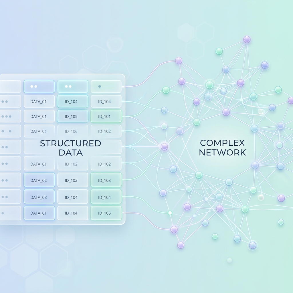
With the nodes instantiated and the relationships forged, your Knowledge Graph comes to life. What used to be rows in an export or nested JSON objects is now a rich, visual map of your entire enterprise ecosystem.
What’s Next?
Our enterprise logic is now mathematically modeled in a graph database. The next step? Giving it a proxy to speak!
In our next follow-up, we will explore Connecting Neo4j to Copilot (or Claude), detailing how to utilize the Model Context Protocol (MCP) to let your AI agents query your new architecture graph in natural language.